PISCOLA Fits

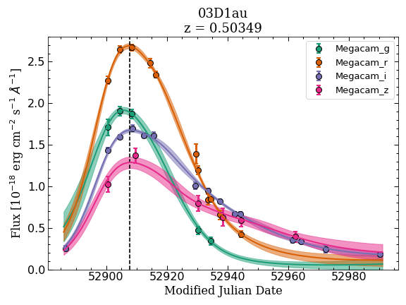
Caption: Gaussian Process (GP) fit of the multi-colour light curves of SN 03D1au. A Matérn-5/2 kernel was used in this case. The solid lines show the mean of the GP fits while the shaded areas represent one standard deviation (1-$\sigma$). The vertical dashed black line marks the initial estimation of $B$-band peak.

Author: Tomás E. Müller-Bravo

Affiliation: University of Southampton

Original Image: link

import matplotlib.pyplot as plt
import numpy as np

# This code is extracted from PISCOLA (https://github.com/temuller/piscola, piscola/sn.py).
# The function that makes this plot is inside a Class (a Type Ia Supernova object). This is a modified version of the actual code.

#set colour palette
new_palette = [plt.get_cmap('Dark2')(i) for i in np.arange(8)] + [plt.get_cmap('Set1')(i) for i in np.arange(8)]

# extract the power of the scientific notation of the flux to normalize the values
exp = np.round(np.log10(np.abs(self.data[self.bands[0]]['flux']).mean()), 0)
y_norm = 10**exp

# set the plot limits
plot_lim_vals = [[self.data[band]['flux'].min(), self.data[band]['flux'].max()] for band in self.bands]
plot_lim_vals = np.ndarray.flatten(np.array(plot_lim_vals))/y_norm
ymin_lim = np.r_[plot_lim_vals, 0.0].min()*0.9
if ymin_lim < 0.0:
    ymin_lim *= 1.1/0.9
ymax_lim = plot_lim_vals.max()*1.05

# beginning of the plot
fig, ax = plt.subplots(figsize=(8, 6))

# self.band is a list of observed bands.
# self.data is a dictionary for light curve data with bands as keys and dictionaries as values with 'mjd', 'flux' and 'std' as keys.
# self.lc_fits is the same as self.data, but for the light curve fits.
for i, band in enumerate(self.bands):

	# extract values for plotting	
	time, flux, std = np.copy(self.lc_fits[band]['mjd']), np.copy(self.lc_fits[band]['flux']), np.copy(self.lc_fits[band]['std'])
	data_time, data_flux, data_std = np.copy(self.data[band]['mjd']), np.copy(self.data[band]['flux']), np.copy(self.data[band]['flux_err'])

	# normalize values
	flux, std = flux/y_norm, std/y_norm
	data_flux, data_std = data_flux/y_norm, data_std/y_norm

	ax.errorbar(data_time, data_flux, data_std, fmt='o', mec='k', capsize=3, capthick=2, ms=8,
		    elinewidth=3, color=new_palette[i],label=band)
	ax.plot(time, flux,'-', color=new_palette[i], lw=2, zorder=16)
	ax.fill_between(time, flux-std, flux+std, alpha=0.5, color=new_palette[i])
	# 'exp' is used here to include it in the label for aesthetic purposes
	ax.set_ylabel(r'Flux [10$^{%.0f}$ erg cm$^{-2}$ s$^{-1}$ $\AA^{-1}$]'%exp, fontsize=16, family='serif')

# self.tmax is the estimated time of the rest-frame B-band peak luminosity
ax.axvline(x=self.tmax, color='k', linestyle='--')
ax.minorticks_on()
ax.tick_params(which='major', length=6, width=1, direction='in', top=True, right=True, labelsize=16)
ax.tick_params(which='minor', length=3, width=1, direction='in', top=True, right=True, labelsize=16)
ax.set_xlabel('Modified Julian Date', fontsize=16, family='serif')
# self.name is the name of the Supernova and self.z is the redshift
ax.set_title(f'{self.name}\nz = {self.z:.5}', fontsize=18, family='serif')
ax.legend(fontsize=13, loc='upper right')
ax.set_ylim(ymin_lim, ymax_lim)
plt.show()

Press the tag below to see more examples