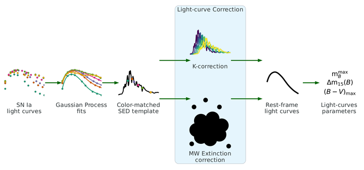
PISCOLA Flowchart

Caption: Flowchart of the main procedures in PISCOLA. Gaussian Process is used to fit the light curves of SNe Ia. Afterwards, an SED template is warped to match the observed SN colors, which is then corrected for redshift (K-correction) and Milky Way dust extinction. Finally, rest-frame light curves are obtained and the light-curve parameters are estimated.
Author: Tomás E. Müller-Bravo
Affiliation: University of Southampton
# Here I used the diagrams package (https://github.com/mingrammer/diagrams). I created my own node (following
# the same structures as the other ones) to add my own images to the diagram. Check the website
# (https://diagrams.mingrammer.com) for more examples.

from diagrams import Diagram
from diagrams.piscola.lightcurves import Lightcurves, Fits, SEDMatch, Kcorr, Dust, Bband, LcParams
from diagrams import Cluster


# Attributes
graph_attr = {
    "fontsize": "40",
    "compund": "True",
    "margin": "-1.8"
}

node_attr = {
    "fontsize": "20",
    "fixedsize": "True",
    "width": "2",
    "height": "2",
    "margin": "0.5",
}

cluster_attr = {
    "fontsize": "20",
}

edge_attr = {
    "minlen": "1.0",
    "penwidth":"3.0",
    "concentrate": "true",
    "color": "darkgreen"
}


with Diagram("", filename='piscola_flowchart', show=False, direction='LR',
             node_attr=node_attr, graph_attr=graph_attr, edge_attr=edge_attr, outformat='pdf') as diag:
    net = Lightcurves("\n\nSN Ia\nlight curves") >> Fits("\n\nGaussian Process\nfits")

    net2 = net >> SEDMatch("\n\nColor-matched\nSED template")

    with Cluster("Light-curve Correction", graph_attr=cluster_attr):
        kcor = Kcorr("\n\nK-correction")
        lc_corr = [kcor, Dust("\n\n\n\nMW Extinction\ncorrection")]

    lc_params = LcParams("\n\nLight-curves\nparameters")
    net2 >>  lc_corr >> Bband("\n\nRest-frame\nlight curves") >> lc_params #>> kcor


diag
Press the tag below to see more examples